MiniTuring (p46)
The ladder of causation
|
|
|


Authors: Aymen Merrouche and Pierre-Henri Wuillemin.
This notebook follows the example from “The Book Of Why” (Pearl, 2018) chapter 1 page 046
In [1]:
import pyagrum as gum
import pyagrum.lib.notebook as gnb
import pyagrum.causal as csl
import pyagrum.causal.notebook as cslnb
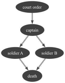
In order for a prisoner to be executed, a certain chain of events must take place. First, the court gives the execution order to the captain. Then, the captain gives the signal to the firing squad (two soldiers A and B) to shoot the prisoner. Finally, the soldiers obey the commandment and shoot at the prisoner.
We create the causal diagram:
The corresponding causal diagram is the following:
In [2]:
mtt = gum.fastBN("court order->captain->soldier A->death<-soldier B<-captain")
mtt
Out[2]:
In [3]:
# filling the CPTs
def smallPertubation(cpt, epsilon=0.0001):
  cpt.fillWith(cpt.translate(epsilon).normalizeAsCPT())


mtt.cpt("court order")[:] = [0.5, 0.5]

# The captain will give the signal only if the court gives the order.
mtt.cpt("captain")[{"court order": 0}] = [1, 0]
mtt.cpt("captain")[{"court order": 1}] = [0, 1]

# The soldiers only fire if the captain gives them the signal.
mtt.cpt("soldier A")[{"captain": 0}] = [1, 0]  # c=0
mtt.cpt("soldier A")[{"captain": 1}] = [0, 1]  # c=1
smallPertubation(mtt.cpt("soldier A"))

mtt.cpt("soldier B")[{"captain": 0}] = [1, 0]  # c=0
mtt.cpt("soldier B")[{"captain": 1}] = [0, 1]  # c=1
smallPertubation(mtt.cpt("soldier B"))

# It only takes one of the two soldiers to shoot for the prisoner to die.
mtt.cpt("death")[{"soldier A": 0, "soldier B": 0}] = [1, 0]  # a=0,b=0
mtt.cpt("death")[{"soldier A": 0, "soldier B": 1}] = [0, 1]  # a=0,b=1
mtt.cpt("death")[{"soldier A": 1, "soldier B": 0}] = [0, 1]  # a=1,b=0
mtt.cpt("death")[{"soldier A": 1, "soldier B": 1}] = [0, 1]  # a=1,b=1
smallPertubation(mtt.cpt("death"))
In [4]:
gnb.sideBySide(
  mtt,
  mtt.cpt("court order"),
  mtt.cpt("captain"),
  mtt.cpt("soldier A"),
  mtt.cpt("soldier B"),
  mtt.cpt("death"),
  captions=[
    "the BN",
    "the marginal for $court order$",
    "the CPT for $captain$",
    "the CPT for $soldier A$",
    "the CPT for $soldier B$",
    "the CPT for $death$",
  ],
)
In [5]:
# gum.saveBN(mtt,os.path.join("out","MiniTuringTest.o3prm"))
1- Answering observational queries (rung one of the ladder of causation) :
If the prisoner is dead, does that mean the court order was given?
i.e. We are interested in distribution:
In [6]:
# inference engine : LazyPropagation
ie = gum.LazyPropagation(mtt)

# Knowing that death = 1
ie.setEvidence({"death": 1})
ie.makeInference()
gnb.sideBySide(
  ie.posterior("court order"),
  gnb.getInference(mtt, evs={"death": 1}),
  captions=["$P(court order|death=1)", "Complete inference with evidence={deah:1}"],
)
If the prisoner is dead, this means that both soldiers fired, the captain gave the signal to the firing squad and the court ordered the execution.
Suppose we find out that A fired. What does that tell us about B?
i.e. We are interested in distribution:
In [7]:
gnb.showInference(mtt, evs={"soldier A": 1})

Following the diagram, we can say that B fired too since A wouldn’t have fired if the captain didn’t give the signal.
2- Answering interventional queries (rung two of the ladder of causation) :
Consists of predicting the effect of a deliberate intervention What would $ X $ be, if I do $ Y $? (i.e. \(P(X \mid do(Y))\)) Interventional queries can not be answered using only passively collected data.
In [8]:
mttModele = csl.CausalModel(mtt)
gum.config.push()
gum.config["notebook", "graph_format"] = "png"
gnb.show(mttModele)
gum.config.pop()
What if Soldier A decides on his own initiative to fire, without waiting for the captain’s command? Will the prisoner be dead or alive?
In [9]:
# We do(soldier A = 1) (a deliberate intervention)
cslnb.showCausalImpact(mttModele, "death", doing="soldier A", values={"soldier A": 1})
|
|
|
|---|---|
| 0.0001 | 0.9999 |
Even if the captain didn’t give the command to the firing squad, the prisoner still died we soldier A decided to shoot him.
Subset {captain} meets the back-door criterion relative to (soldier A, death) because:
1- no node in {captain} is a descendant of “soldier A”
2- {captain} blocks every path between “soldier A” and “death” that contains an arrow into “death”
So {captain} satisfies the back-door criterion relative to (soldier A, death), the causal effect of “soldier A” over “death” is given by the formula
\[P(death ∣ do(soldierA = 1)) = \sum_{captain}{P(death ∣ captain,soldierA).P(captain)}\]
What if Soldier A decides on his own initiative to fire, without waiting for the captain’s command? What does that tell us about Soldier B?
In [10]:
# We do(soldier A = 1) (a deliberate intervention)
cslnb.showCausalImpact(mttModele, on="soldier B", doing="soldier A", values={"soldier A": 1})
|
|
|
|---|---|
| 0.5000 | 0.5000 |
A’s spontaneous decision shouldn’t affect variables in the model that are not descendants of A. If we see that A shot, we conclude that B shot too (he wouldn’t have shot without the captain’s order). But if we make A shoot spontaneously without waiting for the captain’s order, we have no information about B. This is the difference between seeing and doing.
What if the captain decides on his own initiative to give the firing order, without waiting for the court order’s command?
In [11]:
mttModele = csl.CausalModel(mtt)
# We do(soldier A = 1) (a deliberate intervention)
cslnb.showCausalImpact(mttModele, "death", doing="captain", values={"captain": 1})
|
|
|
|---|---|
| 0.0001 | 0.9999 |
Subset {soldier A, soldier B} meets the front-door criterion relative to (captain, death) because:
1- {soldier A, soldier B} intercepts all directed paths from “captain” to “death”
2- There is no back-door path from “captain” to {soldier A, soldier B}.
3- All back-door paths from {soldier A, soldier B} to “death” are blocked by “captain.”
3- Answering counterfactual queries (rung three of the ladder of causation) :
Consists of reasoning about hypothetical situations What would have happened if?
Suppose the prisoner is lying dead on the ground. From this, we can conclude (using level one) that A shot, B shot, the captain gave the signal, and the court gave the order. But what if A had decided not to shoot? Would the prisoner be alive?
To answer this question we need to compare the real world where the prisoner is lying dead on the ground, A shot, B shot, the captain gave the signal to the firing squad and the court gave the order :
With a counterfactual world where “\(soldier A = 0\)”, and where the arrow leading into A is erased (since he decided on his own not to shoot we emancipate it from the effect of the captain).
In [12]:
mttCounterfactual = gum.BayesNet(mtt)

# The court did give the order
mttCounterfactual.cpt("court order")[:] = [0, 1]


# Soldier A decides not to shoot
mttCounterfactual.cpt("soldier A")[0, :] = [1, 0]  # c=0
mttCounterfactual.cpt("soldier A")[1, :] = [1, 0]  # c=1


# We emancipate soldier A
mttCounterfactual.eraseArc("captain", "soldier A")
In [13]:
gnb.showBNDiff(mtt, mttCounterfactual, size="4")

In [14]:
gnb.sideBySide(
  mttCounterfactual,
  mttCounterfactual.cpt("court order"),
  mttCounterfactual.cpt("captain"),
  mttCounterfactual.cpt("soldier A"),
  mttCounterfactual.cpt("soldier B"),
  mttCounterfactual.cpt("death"),
  captions=[
    "the BN",
    "the marginal for $court order$",
    "the CPT for $captain$",
    "the CPT for $soldier A$",
    "the CPT for $soldier B$",
    "the CPT for $death$",
  ],
)
In [15]:
gnb.showInference(mttCounterfactual)

Even if A decides not to shoot in the counterfactual world, the court did give the order to the captain who gave the signal to the firing squad including A who decided not to shoot, however, B shot and killed the prisoner.
Mathematically, this counterfactual is the following conditional probability:
where variables with a subscript C are unobserved (and unobservable) variables that live in the counterfactual world, while variables without subscript are observable.
In [ ]: