Learning classifiers

In [1]:

import pyagrum.skbn as skbn
import pyagrum.lib.notebook as gnb

skbn is a pyAgrum’s module that allows to use bayesian networks as classifier in the scikit-learn environment. ## Initialization of parameters

First, we initialize the parameters to indicate properties we want our classifier to have.

In [2]:

BNTest = skbn.createBNClassifier(
  learningMethod="Chow-Liu",
  prior="Smoothing",
  priorWeight=0.5,
  discretizationStrategy="quantile",
  usePR=True,
  significant_digit=13,
)

Then, we train the classifier thanks to two types of objects.

Learn from csv file

In [3]:

BNTest.fitFromTabular(data="res/creditCardTest.csv", targetName="Class")

Out[3]:

BNClassifier(learningMethod='Chow-Liu', prior='Smoothing', priorWeight=0.5,
             significant_digit=13,
             type_processor=<pyagrum.lib.discreteTypeProcessor.DiscreteTypeProcessor object at 0x113dc6660>,
             usePR=True)

In a Jupyter environment, please rerun this cell to show the HTML representation or trust the notebook.
On GitHub, the HTML representation is unable to render, please try loading this page with nbviewer.org.

BNClassifier

iFitted

Parameters

	type_processor	<pyagrum.lib....t 0x113dc6660>
	learningMethod	'Chow-Liu'
	prior	'Smoothing'
	priorWeight	0.5
	usePR	True
	significant_digit	13
	scoringType	'BIC'
	constraints	None
	possibleSkeleton	None
	DirichletCsv	None
	beta	1

Fitted attributes

Name	Type	Value
MarkovBlanket_	BayesNet	(pyagrum.Baye...: 9, mem: 96o}
bn_	BayesNet	(pyagrum.Baye...mem: 5Ko 776o}
classes_	ndarray[float64](2,)	[0.,1.]
feature_names_in_	ndarray[object](30,)	['Time','V1','V2',...,'V27','V28','Amount']
fromModel_	bool	False
label_	str	'1.0'
learner_	BNLearner	(pyagrum.BNLe... : 0.500000
n_features_in_	int	30
targetType_	Float64DType	dtype('float64')
target_	str	'Class'
threshold_	float64	0.121
variableNameIndexDictionary_	dict	{'Amount': 29, 'Time': 0, 'V1': 1, 'V10': 10, ...}

In [4]:

for i in BNTest.bn_.nodes():
  print(BNTest.bn_.variable(i))

Class:Labelized({0.0|1.0})
Time:Discretized(<(0;1578[,[1578;3733[,[3733;6982[,[6982;11033[,[11033;170348)>)
V1:Discretized(<(-30.55238004;-1.332949264[,[-1.332949264;-0.654664391[,[-0.654664391;0.30537512[,[0.30537512;1.183457866[,[1.183457866;2.132386021)>)
V2:Discretized(<(-25.64052693;-0.362407881[,[-0.362407881;0.104021894[,[0.104021894;0.582468095[,[0.582468095;1.126264537[,[1.126264537;22.05772899)>)
V3:Discretized(<(-31.10368482;0.107723002[,[0.107723002;0.675277319[,[0.675277319;1.145250512[,[1.145250512;1.731063013[,[1.731063013;4.101716178)>)
V4:Discretized(<(-4.657545034;-0.8356831[,[-0.8356831;0.033423475[,[0.033423475;0.648385592[,[0.648385592;1.445625927[,[1.445625927;12.11467184)>)
V5:Discretized(<(-22.10553152;-0.8136663[,[-0.8136663;-0.355922897[,[-0.355922897;0.03294682[,[0.03294682;0.534604692[,[0.534604692;11.97426887)>)
V6:Discretized(<(-7.574798166;-0.789777644[,[-0.789777644;-0.370597233[,[-0.370597233;0.035355351[,[0.035355351;0.711815449[,[0.711815449;10.03392286)>)
V7:Discretized(<(-43.55724157;-0.691953395[,[-0.691953395;-0.264737855[,[-0.264737855;0.111993062[,[0.111993062;0.576160082[,[0.576160082;12.21924885)>)
V8:Discretized(<(-41.04426092;-0.248777743[,[-0.248777743;-0.061897336[,[-0.061897336;0.101158949[,[0.101158949;0.417327159[,[0.417327159;20.00720837)>)
V9:Discretized(<(-13.43406632;-0.258885741[,[-0.258885741;0.43278337[,[0.43278337;1.003150701[,[1.003150701;1.606746899[,[1.606746899;10.39288882)>)
V10:Discretized(<(-24.58826244;-0.887241636[,[-0.887241636;-0.486914228[,[-0.486914228;-0.174270174[,[-0.174270174;0.281998033[,[0.281998033;12.25994935)>)
V11:Discretized(<(-2.595325047;-0.216850152[,[-0.216850152;0.467606404[,[0.467606404;1.069280983[,[1.069280983;1.894362474[,[1.894362474;12.01891318)>)
V12:Discretized(<(-18.68371463;-2.603364421[,[-2.603364421;-1.98917204[,[-1.98917204;-1.010277351[,[-1.010277351;0.297745303[,[0.297745303;3.774837253)>)
V13:Discretized(<(-3.389510119;-0.277525814[,[-0.277525814;0.487335344[,[0.487335344;1.191999923[,[1.191999923;1.871678101[,[1.871678101;4.465413177)>)
V14:Discretized(<(-19.21432549;-0.198436291[,[-0.198436291;0.394380416[,[0.394380416;1.129212699[,[1.129212699;1.560400117[,[1.560400117;5.7487338)>)
V15:Discretized(<(-4.498944677;-0.89821835[,[-0.89821835;-0.252119146[,[-0.252119146;0.228108992[,[0.228108992;0.673845558[,[0.673845558;2.533660621)>)
V16:Discretized(<(-14.12985452;-0.73752994[,[-0.73752994;-0.191439365[,[-0.191439365;0.226074322[,[0.226074322;0.649708023[,[0.649708023;3.930881236)>)
V17:Discretized(<(-25.16279937;-0.373269972[,[-0.373269972;0.063135741[,[0.063135741;0.445363418[,[0.445363418;0.906547825[,[0.906547825;7.893392532)>)
V18:Discretized(<(-9.498745921;-0.642528115[,[-0.642528115;-0.1793428[,[-0.1793428;0.166270273[,[0.166270273;0.556347095[,[0.556347095;4.115559919)>)
V19:Discretized(<(-4.932733055;-0.673232673[,[-0.673232673;-0.228782999[,[-0.228782999;0.150300643[,[0.150300643;0.636971987[,[0.636971987;5.22834179)>)
V20:Discretized(<(-13.27603434;-0.183661648[,[-0.183661648;-0.067770251[,[-0.067770251;0.044433337[,[0.044433337;0.232763125[,[0.232763125;11.05900429)>)
V21:Discretized(<(-22.79760391;-0.298193493[,[-0.298193493;-0.179496901[,[-0.179496901;-0.054862175[,[-0.054862175;0.105119219[,[0.105119219;27.20283916)>)
V22:Discretized(<(-8.887017141;-0.649013527[,[-0.649013527;-0.291807777[,[-0.291807777;0.009627985[,[0.009627985;0.351257859[,[0.351257859;8.361985192)>)
V23:Discretized(<(-19.25432762;-0.215264519[,[-0.215264519;-0.092460674[,[-0.092460674;-1.53e-05[,[-1.53e-05;0.122578904[,[0.122578904;13.87622086)>)
V24:Discretized(<(-2.51237651;-0.441546648[,[-0.441546648;-0.013724876[,[-0.013724876;0.248363887[,[0.248363887;0.468668566[,[0.468668566;3.200201195)>)
V25:Discretized(<(-4.781605522;-0.238381673[,[-0.238381673;0.02446896[,[0.02446896;0.212093775[,[0.212093775;0.411607181[,[0.411607181;5.525092704)>)
V26:Discretized(<(-1.338556498;-0.390763459[,[-0.390763459;-0.124995177[,[-0.124995177;0.128836809[,[0.128836809;0.664810252[,[0.664810252;3.517345612)>)
V27:Discretized(<(-7.976099818;-0.097082439[,[-0.097082439;-0.025569225[,[-0.025569225;0.034724233[,[0.034724233;0.216123366[,[0.216123366;4.173387153)>)
V28:Discretized(<(-3.054084903;-0.043029565[,[-0.043029565;0.006334972[,[0.006334972;0.029936485[,[0.029936485;0.111331248[,[0.111331248;4.860769069)>)
Amount:Discretized(<(0;2.78[,[2.78;11.66[,[11.66;25.52[,[25.52;73.5[,[73.5;4002.88)>)

In [5]:

gnb.sideBySide(BNTest.bn_, gnb.getInference(BNTest.bn_, size="15!"))

In [6]:

gnb.showBN(BNTest.MarkovBlanket_)

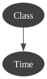
../_images/notebooks_51-Classifier_Learning_11_0.svg

Learn from array-likes

We use a method to transform the csv file in two array-likes in order to train from the same database.

In [7]:

# we use now another method to learn the BN (MIIC)
BNTest = skbn.createBNClassifier(
  learningMethod="MIIC",
  prior="Smoothing",
  priorWeight=0.5,
  discretizationStrategy="quantile",
  usePR=True,
  significant_digit=13,
)

xTrain, yTrain = BNTest.XYfromCSV(filename="res/creditCardTest.csv", target="Class")

In [8]:

BNTest.fit(xTrain, yTrain)

Out[8]:

BNClassifier(prior='Smoothing', priorWeight=0.5, significant_digit=13,
             type_processor=<pyagrum.lib.discreteTypeProcessor.DiscreteTypeProcessor object at 0x114dd5220>,
             usePR=True)

In a Jupyter environment, please rerun this cell to show the HTML representation or trust the notebook.
On GitHub, the HTML representation is unable to render, please try loading this page with nbviewer.org.

BNClassifier

iFitted

Parameters

	type_processor	<pyagrum.lib....t 0x114dd5220>
	prior	'Smoothing'
	priorWeight	0.5
	usePR	True
	significant_digit	13
	learningMethod	'MIIC'
	scoringType	'BIC'
	constraints	None
	possibleSkeleton	None
	DirichletCsv	None
	beta	1

Fitted attributes

Name	Type	Value
MarkovBlanket_	BayesNet	(pyagrum.Baye...m: 293Ko 288o}
bn_	BayesNet	(pyagrum.Baye...Mo 117Ko 968o}
classes_	ndarray[float64](2,)	[0.,1.]
feature_names_in_	ndarray[object](30,)	['Time','V1','V2',...,'V27','V28','Amount']
fromModel_	bool	False
label_	str	'1.0'
learner_	BNLearner	(pyagrum.BNLe... : 0.500000
n_features_in_	int	30
targetType_	Float64DType	dtype('float64')
target_	str	'Class'
threshold_	float64	0.5612
variableNameIndexDictionary_	dict	{'Amount': 29, 'Time': 0, 'V1': 1, 'V10': 10, ...}

In [9]:

gnb.showBN(BNTest.bn_)

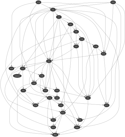
../_images/notebooks_51-Classifier_Learning_16_0.svg

In [10]:

gnb.showBN(BNTest.MarkovBlanket_)

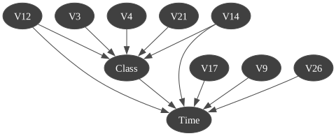
../_images/notebooks_51-Classifier_Learning_17_0.svg

Create a classifier from a Bayesian network

If we already have a Bayesian network with learned parameters, we can create a classifier that uses it. In this case we do not have to train the classifier on data since it the Bayesian network is already trained.

In [11]:

ClassfromBN = skbn.createBNClassifier(significant_digit=7)

In [12]:

ClassfromBN.fromTrainedModel(
  bn=BNTest.bn_,
  targetAttribute="Class",
  targetModality="1.0",
  threshold=BNTest.threshold_,
  variableList=xTrain.columns.tolist(),
)

In [13]:

gnb.showBN(ClassfromBN.bn_)

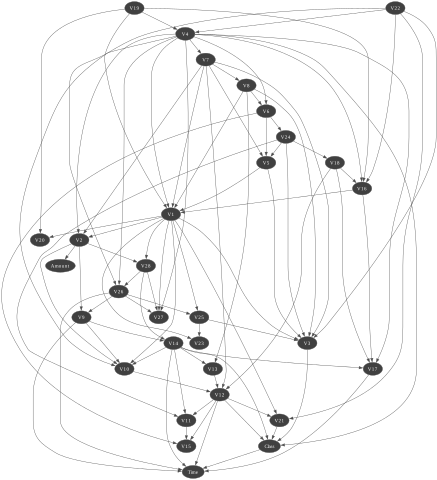
../_images/notebooks_51-Classifier_Learning_22_0.svg

In [14]:

gnb.showBN(ClassfromBN.MarkovBlanket_)

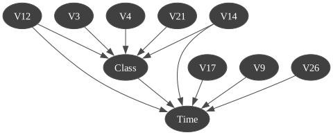
../_images/notebooks_51-Classifier_Learning_23_0.svg

Then, we work with functions from scikit-learn like score. We can also call it with a csv file or two array-likes.

In [15]:

xTest, yTest = ClassfromBN.XYfromCSV(filename="res/creditCardTest.csv", target="Class")

Prediction for classifier

Prediction with csv file

In [16]:

scoreCSV1 = BNTest.score("res/creditCardTest.csv", y=yTest)
print("{0:.2f}% good predictions".format(100 * scoreCSV1))

99.77% good predictions

In [17]:

scoreCSV2 = ClassfromBN.score("res/creditCardTest.csv", y=yTest)
print("{0:.2f}% good predictions".format(100 * scoreCSV2))

99.77% good predictions

Prediction with array-like

In [18]:

scoreAR1 = BNTest.score(xTest, yTest)
print("{0:.2f}% good predictions".format(100 * scoreAR1))

99.77% good predictions

In [19]:

scoreAR2 = ClassfromBN.score(xTest, yTest)
print("{0:.2f}% good predictions".format(100 * scoreAR2))

99.77% good predictions

ROC and Precision-Recall curves with all methods

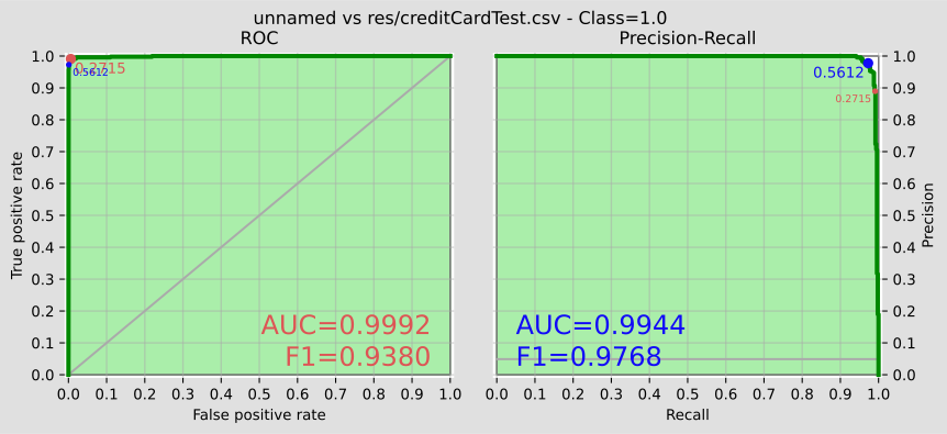
In addition (and of course), we can work with functions from pyagrum (from pyagrum.lib.bn2roc).

In [20]:

BNTest.showROC_PR("res/creditCardTest.csv")

../_images/notebooks_51-Classifier_Learning_34_0.svg

In [ ]: