Using sklearn to cross-validate bayesian network classifier

Overview

BNClassifier from pyagrum.skbn is a Bayesian Network-based classifier compatible with the scikit-learn API. This means you can use it with all standard sklearn tools such as train_test_split, cross_validate, accuracy_score, confusion_matrix, and more.

This notebook demonstrates four typical use cases on the Iris dataset (3 classes, 4 continuous features):

1. ``fit(X, y)`` — Standard sklearn training from a feature matrix and a label vector

2. ``fitFromData(df, targetName)`` — Training directly from a pandas DataFrame or a CSV file

3. ``fromTrainedModel(bn, targetAttribute)`` — Wrapping an existing pyAgrum Bayesian network into a sklearn-compatible classifier

4. Cross-validation — Using sklearn’s cross_validate to get a robust performance estimate

from pyagrum.skbn import createBNClassifier

from sklearn import datasets
from sklearn.model_selection import train_test_split, cross_validate
from sklearn.metrics import (
  accuracy_score,
  confusion_matrix,
  classification_report,
  ConfusionMatrixDisplay,
)

import pandas as pd
import matplotlib.pyplot as plt

1. Loading the Iris Dataset

The Iris dataset is one of the most well-known classification benchmarks. It contains 150 samples described by 4 continuous measurements:

• sepal length and width (cm)

• petal length and width (cm)

The target variable has 3 classes (setosa, versicolor, virginica).

Since the features are continuous, BNClassifier will automatically discretize them into bins before learning the structure of the Bayesian network.

# Load the Iris dataset
iris = datasets.load_iris()
X = iris.data  # shape (150, 4) — continuous features
y = iris.target  # 0: setosa, 1: versicolor, 2: virginica

print(f"Samples  : {X.shape[0]}")
print(f"Features : {X.shape[1]}  →  {iris.feature_names}")
print(f"Classes  : {len(iris.target_names)}  →  {iris.target_names.tolist()}")

Samples  : 150
Features : 4  →  ['sepal length (cm)', 'sepal width (cm)', 'petal length (cm)', 'petal width (cm)']
Classes  : 3  →  ['setosa', 'versicolor', 'virginica']

model = createBNClassifier(
  learningMethod="MIIC",
  prior="Smoothing",
  priorWeight=1,
  discretizationNbBins=3,
  discretizationStrategy="kmeans",
  discretizationThreshold=10,
)

2. Training and Evaluating the Classifier

We define a BNClassifier using the MIIC structure learning algorithm and k-means discretization into 3 bins. A Smoothing prior is added to avoid zero probabilities in the conditional probability tables.

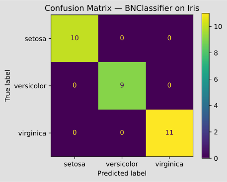
The dataset is split into a training set (80%) and a test set (20%). The classifier is then trained with fit(X_train, y_train) — the standard sklearn interface — and evaluated using accuracy_score, classification_report, and a confusion matrix.

# Split into training (80%) and test (20%) sets
X_train, X_test, y_train, y_test = train_test_split(X, y, test_size=0.2, random_state=42)

# Train the classifier
model.fit(X_train, y_train)

# Predict on the test set
y_pred = model.predict(X_test)

# Overall accuracy
print(f"Accuracy: {accuracy_score(y_test, y_pred):.4f}\n")

# Per-class precision, recall and F1-score
print("Classification Report:")
print(classification_report(y_test, y_pred, target_names=iris.target_names))

# Confusion matrix
fig, ax = plt.subplots(figsize=(5, 4))
ConfusionMatrixDisplay.from_predictions(y_test, y_pred, display_labels=iris.target_names, ax=ax)
ax.set_title("Confusion Matrix — BNClassifier on Iris")
plt.tight_layout()
plt.show()

Accuracy: 1.0000

Classification Report:
              precision    recall  f1-score   support

      setosa       1.00      1.00      1.00        10
  versicolor       1.00      1.00      1.00         9
   virginica       1.00      1.00      1.00        11

    accuracy                           1.00        30
   macro avg       1.00      1.00      1.00        30
weighted avg       1.00      1.00      1.00        30

3. Loading Data with fitFromTabular

The fitFromTabular(data, targetName) method offers a more convenient interface when data is already in tabular form. Instead of separating features and labels manually, you pass either:

• a pandas DataFrame with a named column for the target, or

• a CSV file path along with the name of the target column.

This avoids the manual X = df.drop(...) / y = df[...] split required by the standard sklearn fit(X, y).

# Build a DataFrame from the training set only (features + target column)
df_train = pd.DataFrame(X_train, columns=iris.feature_names)
df_train["species"] = y_train

# Train using fitFromTabular — target column is identified by name
model2 = createBNClassifier(
  learningMethod="MIIC",
  prior="Smoothing",
  priorWeight=1,
  discretizationNbBins=3,
  discretizationStrategy="kmeans",
  discretizationThreshold=10,
)
model2.fitFromTabular(df_train, targetName="species")

# Evaluate on the test set (features only, passed as a DataFrame)
X_test_df = pd.DataFrame(X_test, columns=iris.feature_names)
y_pred2 = model2.predict(X_test_df)
print(f"Accuracy with fitFromTabular: {accuracy_score(y_test, y_pred2):.4f}")

Accuracy with fitFromTabular: 1.0000

4. Building a Classifier from a Pre-trained Bayesian Network

If you already have a trained Bayesian network — learned externally or provided by a domain expert — you can wrap it into a BNClassifier using fromTrainedModel.

The resulting object is fully sklearn-compatible: you can call predict, predict_proba, and use it in pipelines or cross-validation.

Here we reuse the Bayesian network learned in section 2 to create a new classifier without re-training.

# Retrieve the Bayesian network learned in section 2
bn = model.bn_
target = model.target_  # "y" — the name assigned to the target variable during fit

# Wrap the pre-trained network into a new BNClassifier
# dtype=int ensures predictions are returned as integers, matching the original target type
model3 = createBNClassifier()
model3.fromTrainedModel(bn, targetAttribute=target, dtype=int)

# Predict on the same test set
y_pred3 = model3.predict(X_test)
print(f"Accuracy with fromTrainedModel: {accuracy_score(y_test, y_pred3):.4f}")

Accuracy with fromTrainedModel: 0.2333

5. Cross-Validation

One of the main advantages of the sklearn-compatible API is the ability to use cross_validate directly. This performs k-fold cross-validation and returns the score for each fold, giving a more robust performance estimate than a single train/test split.

We run the cross-validation with cv=30 and cv=50 folds on the full Iris dataset.

# 30-fold cross-validation
cv_30 = cross_validate(model, X, y, cv=30)
print(f"Fold scores   (cv=30) : {cv_30['test_score']}")
print(f"Mean accuracy (cv=30) : {cv_30['test_score'].mean():.4f}")

Fold scores   (cv=30) : [1.  1.  1.  1.  1.  1.  1.  1.  1.  1.  0.8 1.  1.  1.  0.8 1.  1.  0.8
 1.  1.  1.  0.8 1.  1.  1.  1.  1.  1.  1.  1. ]
Mean accuracy (cv=30) : 0.9733

# 50-fold cross-validation
cv_50 = cross_validate(model, X, y, cv=50)
print(f"Fold scores   (cv=50) : {cv_50['test_score']}")
print(f"Mean accuracy (cv=50) : {cv_50['test_score'].mean():.4f}")

Fold scores   (cv=50) : [1.         1.         1.         1.         1.         1.
 1.         1.         1.         1.         1.         1.
 1.         1.         1.         1.         1.         1.
 1.         1.         0.66666667 1.         1.         1.
 1.         1.         1.         0.66666667 1.         1.
 1.         1.         1.         0.66666667 1.         1.
 1.         1.         1.         1.         1.         1.
 1.         1.         1.         1.         1.         1.
 1.         1.        ]
Mean accuracy (cv=50) : 0.9800