Multinomial Simpson Paradox

this notebook shows a model for a multinomial Simpson paradox.

import pandas as pd

import pyagrum as gum
import pyagrum.lib.notebook as gnb

Building the models

# building a model including a Simpson's paradox
import scipy.stats as stats

bn = gum.fastBN("A[0,90]->B[0:40:200]<-C[0,5]->A")

bn.cpt("C").fillFromDistribution(stats.uniform, loc=0, scale=5)
bn.cpt("A").fillFromDistribution(stats.uniform, loc="C*12", scale=30)
bn.cpt("B").fillFromDistribution(stats.norm, loc="5+C*4-int(A/8)", scale=3);

As a site note we are dealing here with quite large models already :

bn.memoryFootprint()

878016

help(bn.memoryFootprint)

Help on method memoryFootprint in module pyagrum.pyagrum:

memoryFootprint() -> int method of pyagrum.pyagrum.BayesNet instance
    Returns the memory footprint in bytes of the Bayesian network.

    Returns
    -------
    int
      the memory footprint in bytes of the Bayesian network

#  generating a CSV, taking this model as the causal one.
gum.generateSample(bn, 400, "out/sample.csv", with_labels=False)
df = pd.read_csv("out/sample.csv")
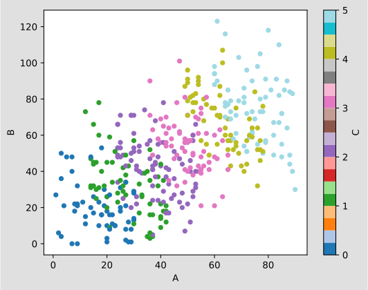
df.plot.scatter(x="A", y="B", c="C", colormap="tab20");

cm = gum.CausalModel(bn)
_, p, _ = gum.causalImpact(cm, on="B", doing="A")

# building an Markov-equivalent model, generating a CSV, taking this model as the causal one.
bn2 = gum.BayesNet(bn)
bn2.reverseArc("C", "A")
bn2

gum.generateSample(bn2, 400, "out/sample2.csv", with_labels=False)
df2 = pd.read_csv("out/sample2.csv")

cm2 = gum.CausalModel(bn2)
_, p2, _ = gum.causalImpact(cm2, on="B", doing="A")

The observationnal model and its paradoxal structure (exactly the same with the second Markov-equivalent model)

gnb.flow.row(
  gnb.getBN(bn),
  df.plot.scatter(x="A", y="B"),
  df.plot.scatter(x="A", y="B", c="C", colormap="tab20"),
  captions=["the observationnal model", "the trend is increasing", "the trend is decreasing for any value for C !"],
)
gnb.flow.row(
  gnb.getBN(bn2),
  df2.plot.scatter(x="A", y="B"),
  df2.plot.scatter(x="A", y="B", c="C", colormap="tab20"),
  captions=["the Markov-equivalent model", "the trend is increasing", "the trend is decreasing for any value for C !"],
)
gnb.flow.display()

the Markov-equivalent model

the trend is increasing

the trend is decreasing for any value for C !

The paradox is revealed in the trend of the inferred means : the means are increasing with the value of \(A\) except for any value of :math:`C` …

gum.config["notebook", "histogram_epsilon"] = 0.001
gum.config["notebook", "histogram_discretized_scale"] = 0.4

for a in [10, 20, 30]:
  gnb.flow.add_html(gnb.getPosterior(bn, target="B", evs={"A": a}), f"$P(B|A={a})$")
gnb.flow.new_line()
for a in [10, 20, 30]:
  gnb.flow.add_html(gnb.getPosterior(bn, target="B", evs={"A": a, "C": 0}), f"P(B | $A={a},C=0)$")
gnb.flow.new_line()
for a in [10, 20, 30]:
  gnb.flow.add_html(gnb.getPosterior(bn, target="B", evs={"A": a, "C": 2}), f"P(B | $A={a},C=2$)")
gnb.flow.new_line()
for a in [10, 20, 30]:
  gnb.flow.add_html(gnb.getPosterior(bn, target="B", evs={"A": a, "C": 4}), f"P(B | $A={a},C=4$)")
gnb.flow.display()

$P(B|A=10)$

$P(B|A=20)$

$P(B|A=30)$

P(B | $A=10,C=0)$

P(B | $A=20,C=0)$

P(B | $A=30,C=0)$

P(B | $A=10,C=2$)

P(B | $A=20,C=2$)

P(B | $A=30,C=2$)

P(B | $A=10,C=4$)

P(B | $A=20,C=4$)

P(B | $A=30,C=4$)

Now that the paradoxal structure is understood and the paradox is revealed, will we choose to observe \(C\) (or not) before deciding to increase or decrease \(A\) (with the goal to maximize \(B\)) ?

Of course, it depends on the causal structure of the problem !

If \(C\) is cause for \(A\), observing \(C\) really gives a new information about \(B\).

gnb.flow.add_html(gnb.getCausalModel(cm), "the first causal model")
gnb.flow.new_line()
for v in [10, 20, 30]:
  gnb.flow.add_html(gnb.getProba(p.extract({"A": v})), f"Doing $A={v}$")
gnb.flow.display()

the first causal model

Doing $A=10$

Doing $A=20$

Doing $A=30$

if \(A\) is cause for \(C\), observing \(C\) may lead to misinterpretations about the causal role of \(A\).

gnb.flow.add_html(gnb.getCausalModel(cm2), "the second causal model")
gnb.flow.new_line()
for v in [10, 20, 30]:
  gnb.flow.add_html(gnb.getProba(p2.extract({"A": v})), f"Doing $A={v}$")
gnb.flow.display()

the second causal model

Doing $A=10$

Doing $A=20$

Doing $A=30$