The Effect of Education and Experience on Salary (p251)

Authors: Aymen Merrouche and Pierre-Henri Wuillemin.

This notebook follows the example from “The Book Of Why” (Pearl, 2018) chapter 8 page 251

Counterfactuals for Education and Salary

import pyagrum as gum
import pyagrum.lib.notebook as gnb

In this example we are interested in the effect of experience and education on the salary of an employee, we are in possession of the following data:

Employé	EX(u)	ED(u)	\(S_{0}(u)\)	\(S_{1}(u)\)	\(S_{2}(u)\)
Alice	8	0	86,000	?	?
Bert	9	1	?	92,500	?
Caroline	9	2	?	?	97,000
David	8	1	?	91,000	?
Ernest	12	1	?	100,000	?
Frances	13	0	97,000	?	?
etc

• \(EX(u)\) : years of experience of employee \(u\). [0,20]

• \(ED(u)\) : Level of education of employee \(u\) (0:high school degree (low), 1:college degree (medium), 2:graduate degree (high)) [0,2]

• \(S_{i}(u)\) [65k,150k] :

  • salary (observable) of employee \(u\) if \(i = ED(u)\),

  • Potential outcome (unobservable) if \(i \not = ED(u)\), salary of employee \(u\) if he had a level of education of \(i\).

We are left with the previous data and we want to answer the counterfactual question What would Alice’s salary be if she attended college ? (i.e. \(S_{1}(Alice)\))

A Causal model

In this model it is assumed that an employee’s salary is determined by his level of education and his experience. Years of experience are also affected by the level of education. Having a higher level of education means spending more time studying hence less experience.

edex = gum.fastBN(
  "Ux[-2,10]->experience[0,20]<-education{low|medium|high}->salary[65,150]<-Us[0,25];experience->salary"
)
edex

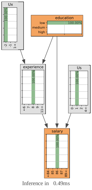
However counterfactual queries are specific to one datapoint (in our case Alice), we need to add additional variables to our model to allow for individual variations:

• Us : unobserved variables that affect salary.[0,25k]

• Ux : unobserved variables that affect experience.[-2,10]

# no prior information about the individual (datapoint)
edex.cpt("Us").fillWith(1).normalize()
edex.cpt("Ux").fillWith(1).normalize()
# education level(supposed)
edex.cpt("education")[:] = [0.4, 0.4, 0.2]

Experience listens to Education and Ux :

\[Ex = 10 -4 \times Ed + Ux\]

edex.cpt("experience").fillFromFunction("10-4*education+Ux")
edex.cpt("experience")

		experience
education	Ux	0	1	2	3	4	5	6	7	8	9	10	11	12	13	14	15	16	17	18	19	20
low	-2	0.0000	0.0000	0.0000	0.0000	0.0000	0.0000	0.0000	0.0000	1.0000	0.0000	0.0000	0.0000	0.0000	0.0000	0.0000	0.0000	0.0000	0.0000	0.0000	0.0000	0.0000
	-1	0.0000	0.0000	0.0000	0.0000	0.0000	0.0000	0.0000	0.0000	0.0000	1.0000	0.0000	0.0000	0.0000	0.0000	0.0000	0.0000	0.0000	0.0000	0.0000	0.0000	0.0000
	0	0.0000	0.0000	0.0000	0.0000	0.0000	0.0000	0.0000	0.0000	0.0000	0.0000	1.0000	0.0000	0.0000	0.0000	0.0000	0.0000	0.0000	0.0000	0.0000	0.0000	0.0000
	1	0.0000	0.0000	0.0000	0.0000	0.0000	0.0000	0.0000	0.0000	0.0000	0.0000	0.0000	1.0000	0.0000	0.0000	0.0000	0.0000	0.0000	0.0000	0.0000	0.0000	0.0000
	2	0.0000	0.0000	0.0000	0.0000	0.0000	0.0000	0.0000	0.0000	0.0000	0.0000	0.0000	0.0000	1.0000	0.0000	0.0000	0.0000	0.0000	0.0000	0.0000	0.0000	0.0000
	3	0.0000	0.0000	0.0000	0.0000	0.0000	0.0000	0.0000	0.0000	0.0000	0.0000	0.0000	0.0000	0.0000	1.0000	0.0000	0.0000	0.0000	0.0000	0.0000	0.0000	0.0000
	4	0.0000	0.0000	0.0000	0.0000	0.0000	0.0000	0.0000	0.0000	0.0000	0.0000	0.0000	0.0000	0.0000	0.0000	1.0000	0.0000	0.0000	0.0000	0.0000	0.0000	0.0000
	5	0.0000	0.0000	0.0000	0.0000	0.0000	0.0000	0.0000	0.0000	0.0000	0.0000	0.0000	0.0000	0.0000	0.0000	0.0000	1.0000	0.0000	0.0000	0.0000	0.0000	0.0000
	6	0.0000	0.0000	0.0000	0.0000	0.0000	0.0000	0.0000	0.0000	0.0000	0.0000	0.0000	0.0000	0.0000	0.0000	0.0000	0.0000	1.0000	0.0000	0.0000	0.0000	0.0000
	7	0.0000	0.0000	0.0000	0.0000	0.0000	0.0000	0.0000	0.0000	0.0000	0.0000	0.0000	0.0000	0.0000	0.0000	0.0000	0.0000	0.0000	1.0000	0.0000	0.0000	0.0000
	8	0.0000	0.0000	0.0000	0.0000	0.0000	0.0000	0.0000	0.0000	0.0000	0.0000	0.0000	0.0000	0.0000	0.0000	0.0000	0.0000	0.0000	0.0000	1.0000	0.0000	0.0000
	9	0.0000	0.0000	0.0000	0.0000	0.0000	0.0000	0.0000	0.0000	0.0000	0.0000	0.0000	0.0000	0.0000	0.0000	0.0000	0.0000	0.0000	0.0000	0.0000	1.0000	0.0000
	10	0.0000	0.0000	0.0000	0.0000	0.0000	0.0000	0.0000	0.0000	0.0000	0.0000	0.0000	0.0000	0.0000	0.0000	0.0000	0.0000	0.0000	0.0000	0.0000	0.0000	1.0000
medium	-2	0.0000	0.0000	0.0000	0.0000	1.0000	0.0000	0.0000	0.0000	0.0000	0.0000	0.0000	0.0000	0.0000	0.0000	0.0000	0.0000	0.0000	0.0000	0.0000	0.0000	0.0000
	-1	0.0000	0.0000	0.0000	0.0000	0.0000	1.0000	0.0000	0.0000	0.0000	0.0000	0.0000	0.0000	0.0000	0.0000	0.0000	0.0000	0.0000	0.0000	0.0000	0.0000	0.0000
	0	0.0000	0.0000	0.0000	0.0000	0.0000	0.0000	1.0000	0.0000	0.0000	0.0000	0.0000	0.0000	0.0000	0.0000	0.0000	0.0000	0.0000	0.0000	0.0000	0.0000	0.0000
	1	0.0000	0.0000	0.0000	0.0000	0.0000	0.0000	0.0000	1.0000	0.0000	0.0000	0.0000	0.0000	0.0000	0.0000	0.0000	0.0000	0.0000	0.0000	0.0000	0.0000	0.0000
	2	0.0000	0.0000	0.0000	0.0000	0.0000	0.0000	0.0000	0.0000	1.0000	0.0000	0.0000	0.0000	0.0000	0.0000	0.0000	0.0000	0.0000	0.0000	0.0000	0.0000	0.0000
	3	0.0000	0.0000	0.0000	0.0000	0.0000	0.0000	0.0000	0.0000	0.0000	1.0000	0.0000	0.0000	0.0000	0.0000	0.0000	0.0000	0.0000	0.0000	0.0000	0.0000	0.0000
	4	0.0000	0.0000	0.0000	0.0000	0.0000	0.0000	0.0000	0.0000	0.0000	0.0000	1.0000	0.0000	0.0000	0.0000	0.0000	0.0000	0.0000	0.0000	0.0000	0.0000	0.0000
	5	0.0000	0.0000	0.0000	0.0000	0.0000	0.0000	0.0000	0.0000	0.0000	0.0000	0.0000	1.0000	0.0000	0.0000	0.0000	0.0000	0.0000	0.0000	0.0000	0.0000	0.0000
	6	0.0000	0.0000	0.0000	0.0000	0.0000	0.0000	0.0000	0.0000	0.0000	0.0000	0.0000	0.0000	1.0000	0.0000	0.0000	0.0000	0.0000	0.0000	0.0000	0.0000	0.0000
	7	0.0000	0.0000	0.0000	0.0000	0.0000	0.0000	0.0000	0.0000	0.0000	0.0000	0.0000	0.0000	0.0000	1.0000	0.0000	0.0000	0.0000	0.0000	0.0000	0.0000	0.0000
	8	0.0000	0.0000	0.0000	0.0000	0.0000	0.0000	0.0000	0.0000	0.0000	0.0000	0.0000	0.0000	0.0000	0.0000	1.0000	0.0000	0.0000	0.0000	0.0000	0.0000	0.0000
	9	0.0000	0.0000	0.0000	0.0000	0.0000	0.0000	0.0000	0.0000	0.0000	0.0000	0.0000	0.0000	0.0000	0.0000	0.0000	1.0000	0.0000	0.0000	0.0000	0.0000	0.0000
	10	0.0000	0.0000	0.0000	0.0000	0.0000	0.0000	0.0000	0.0000	0.0000	0.0000	0.0000	0.0000	0.0000	0.0000	0.0000	0.0000	1.0000	0.0000	0.0000	0.0000	0.0000
high	-2	1.0000	0.0000	0.0000	0.0000	0.0000	0.0000	0.0000	0.0000	0.0000	0.0000	0.0000	0.0000	0.0000	0.0000	0.0000	0.0000	0.0000	0.0000	0.0000	0.0000	0.0000
	-1	0.0000	1.0000	0.0000	0.0000	0.0000	0.0000	0.0000	0.0000	0.0000	0.0000	0.0000	0.0000	0.0000	0.0000	0.0000	0.0000	0.0000	0.0000	0.0000	0.0000	0.0000
	0	0.0000	0.0000	1.0000	0.0000	0.0000	0.0000	0.0000	0.0000	0.0000	0.0000	0.0000	0.0000	0.0000	0.0000	0.0000	0.0000	0.0000	0.0000	0.0000	0.0000	0.0000
	1	0.0000	0.0000	0.0000	1.0000	0.0000	0.0000	0.0000	0.0000	0.0000	0.0000	0.0000	0.0000	0.0000	0.0000	0.0000	0.0000	0.0000	0.0000	0.0000	0.0000	0.0000
	2	0.0000	0.0000	0.0000	0.0000	1.0000	0.0000	0.0000	0.0000	0.0000	0.0000	0.0000	0.0000	0.0000	0.0000	0.0000	0.0000	0.0000	0.0000	0.0000	0.0000	0.0000
	3	0.0000	0.0000	0.0000	0.0000	0.0000	1.0000	0.0000	0.0000	0.0000	0.0000	0.0000	0.0000	0.0000	0.0000	0.0000	0.0000	0.0000	0.0000	0.0000	0.0000	0.0000
	4	0.0000	0.0000	0.0000	0.0000	0.0000	0.0000	1.0000	0.0000	0.0000	0.0000	0.0000	0.0000	0.0000	0.0000	0.0000	0.0000	0.0000	0.0000	0.0000	0.0000	0.0000
	5	0.0000	0.0000	0.0000	0.0000	0.0000	0.0000	0.0000	1.0000	0.0000	0.0000	0.0000	0.0000	0.0000	0.0000	0.0000	0.0000	0.0000	0.0000	0.0000	0.0000	0.0000
	6	0.0000	0.0000	0.0000	0.0000	0.0000	0.0000	0.0000	0.0000	1.0000	0.0000	0.0000	0.0000	0.0000	0.0000	0.0000	0.0000	0.0000	0.0000	0.0000	0.0000	0.0000
	7	0.0000	0.0000	0.0000	0.0000	0.0000	0.0000	0.0000	0.0000	0.0000	1.0000	0.0000	0.0000	0.0000	0.0000	0.0000	0.0000	0.0000	0.0000	0.0000	0.0000	0.0000
	8	0.0000	0.0000	0.0000	0.0000	0.0000	0.0000	0.0000	0.0000	0.0000	0.0000	1.0000	0.0000	0.0000	0.0000	0.0000	0.0000	0.0000	0.0000	0.0000	0.0000	0.0000
	9	0.0000	0.0000	0.0000	0.0000	0.0000	0.0000	0.0000	0.0000	0.0000	0.0000	0.0000	1.0000	0.0000	0.0000	0.0000	0.0000	0.0000	0.0000	0.0000	0.0000	0.0000
	10	0.0000	0.0000	0.0000	0.0000	0.0000	0.0000	0.0000	0.0000	0.0000	0.0000	0.0000	0.0000	1.0000	0.0000	0.0000	0.0000	0.0000	0.0000	0.0000	0.0000	0.0000

Salary listens to Education, Experience and Us :

\[S = 65 + 2.5 \times Ex + 5 \times Ed + Us\]

edex.cpt("salary").fillFromFunction("round(65+2.5*experience+5*education+Us)");

gnb.showInference(edex, size="10")

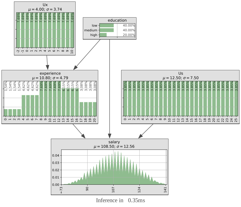
Our question was : What would Alice’s salary be if she attended college ?

To answer this counterfactual question we will follow the three steps algorithm from “The Book Of Why” (Pearl 2018) chapter 8 page 253 :

Step 1 : Abduction for counterfactual

Use the data to retrieve all the information that characterizes Alice

From the data we can retrieve Alice’s profile :

• \(Ed(Alice)\) : 0

• \(Ex(Alice)\) : 8

• \(S_{0}(Alice)\) : 86k

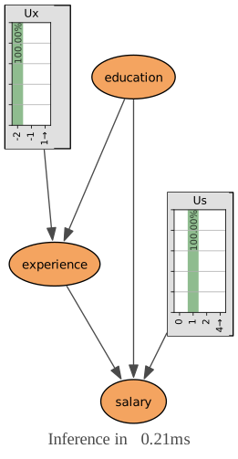
We will use Alice’s profile to get \(U_s\) and \(U_x\), which tell Alice apart from the rest of the data.

ie = gum.LazyPropagation(edex)
ie.setEvidence({"experience": 8, "education": "low", "salary": "86"})
ie.makeInference()
newUs = ie.posterior("Us")
gnb.showProba(newUs)

ie = gum.LazyPropagation(edex)
ie.setEvidence({"experience": 8, "education": "low", "salary": "86"})
ie.makeInference()
newUx = ie.posterior("Ux")
gnb.showProba(newUx)

gnb.showInference(edex, evs={"experience": 8, "education": "low", "salary": "86"}, targets={"Ux", "Us"})

Step 2 & 3 : Action And Prediction for counterfactual

Change the model to match the hypothesis implied by the query (if she had attended university) and then use the data that characterizes Alice to calculate her salary.

We create a counterfactual world with Alice’s idiosyncratic factors, and we operate the intervention:

# the counterfactual world
edexCounterfactual = gum.BayesNet(edex)

# we replace the prior probabilities of idiosyncratic factors with potentials calculated earlier
edexCounterfactual.cpt("Ux").fillWith(newUx)
edexCounterfactual.cpt("Us").fillWith(newUs)
gnb.showInference(edexCounterfactual, size="10")
print("counterfactual world created")

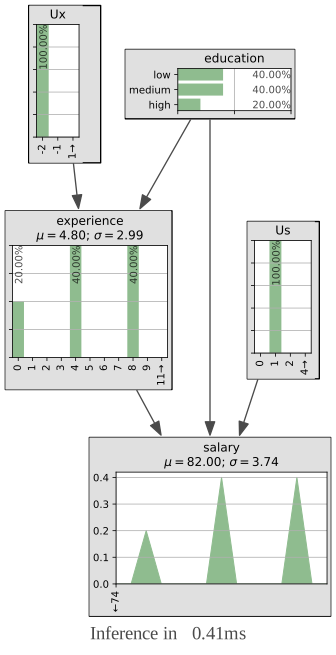
counterfactual world created

# We operate the intervention
edexModele = gum.CausalModel(edexCounterfactual)
gnb.showCausalImpact(edexModele, "salary", doing="education", values={"education": "medium"})

Causal Model

$$ \begin{equation*}P\left(salary \mid \text{do}(education)\right) = P\left(salary\mid education\right)\end{equation*} $$
Explanation : backdoor [] found.

Impact

In the previous query, Alice’s salary if she attended college was lower than her actual salary, that’s because in the counterfactual world where she attended college she had less time to work hence her diminished salary.

We can prove it perfoming a complete inference in the counterfactual world. Since education has no parents in our model (no graph surgery, no causes to emancipate it from), an intervention is equivalent to an observation, the only thing we need to do is to set the value of education:

gnb.showInference(edexCounterfactual, targets={"salary", "experience"}, evs={"education": "medium"}, size="10")

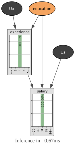
Indeed the expected “experience” decreased.

The result (salary if she had attended college) is given by the formaula:

\[\sum_{salary} salary \times P(salary^* \mid RealSalary = 86k, education = 0, experience = 8, education^*=1)\]

Where variables marked with an asterisk are inobservable.

\[S_1(Alice) = 81k\]

Alice’s salary would be \(\$81\) if she had attended college !

Using pyagrum.counterfactual

In pyAgrum, we can directly use a function that answers counterfactual queries using the previous algorithm.

help(gum.counterfactual)

Help on function counterfactual in module pyagrum.pyagrum:

counterfactual(cm, *, on, whatif, profile=None, values=None)
    Compute a counterfactual distribution using Pearl's twin network method.

    Answers the question: 'Given that we observed *profile*, what would
    *on* have been if *whatif* had been set as specified in *values*?'

    The computation follows the three-step algorithm from Pearl (2018),
    *The Book of Why*, chapter 8: abduction (update parentless node priors
    from the profile), action (apply do(whatif) on the twin model), and
    prediction (evaluate the causal effect on the twin).

    Parameters
    ----------
    cm : pyagrum.CausalModel
        The causal model.
    on : str or set of str
        Target variable(s) of the counterfactual query. A single string is
        automatically converted to a one-element set.
    whatif : str or set of str
        Variable(s) whose values are changed in the counterfactual scenario.
        A single string is automatically converted to a one-element set.
    profile : dict of str → str, optional
        The factual observation as ``{variable_name: value_name}``. This
        grounds the counterfactual (step 1: abduction). Default is empty
        (no factual observation).
    values : dict of str → str, optional
        Counterfactual values for the *whatif* variables as
        ``{variable_name: value_name}``. If omitted, the full distribution
        over all *whatif* values is returned.

    Returns
    -------
    pyagrum.Tensor
        The counterfactual distribution P(on | do(whatif)) evaluated on the
        twin model, optionally sliced by *values*.

    Examples
    --------
    >>> import pyagrum as gum
    >>> bn = pyagrum.BayesNet.fastPrototype('X->Y->Z')
    >>> cm = pyagrum.CausalModel(bn)
    >>> t = pyagrum.counterfactual(cm, on='Z', whatif='X',
    ...                        profile={'Y': 'True'}, values={'X': 'False'})

Let’s try with the previous query

pot = gum.counterfactual(
  cm=gum.CausalModel(edex),
  profile={"experience": 8, "education": "low", "salary": "86"},
  whatif={"education"},
  on={"salary"},
  values={"education": "medium"},
)

gnb.showProba(pot)

We get the same result !

multiple conterfactuals

We get every potential outcome :

pot = gum.counterfactual(
  cm=gum.CausalModel(edex),
  profile={"experience": 8, "education": "low", "salary": "86"},
  whatif={"education"},
  on={"salary"},
)

# pot contains the result for all value of education
for label in pot.variable("education").labels():
  gnb.flow.row(f"for education = {label}", gnb.getProba(pot.extract({"education": label})))

What would Alice’s salary be if she had attended college and had 8 years of experience ?

pot = gum.counterfactual(
  cm=gum.CausalModel(edex),
  profile={"experience": 8, "education": "low", "salary": "86"},
  whatif={"education", "experience"},
  on={"salary"},
  values={"education": "medium", "experience": 8},
)

gnb.showProba(pot)

if she attended college and had 8 years of experience Alice’s salary would be 91k !

In the previous query, Alice’s salary if she attended college was lower than her actual salary, that’s because in the counterfactual world where she attended college she had less time to work hence her diminished salary.

In this query, Alice’s counterfactual salary was higher than her actual salary (+5k corresponding to one level of education), that’s because in the counterfactual world Alice attended college and still had time to work 8 years, so her salary went up.

if she had more experience Some counterfactual can not be computer : With this profile, an experience of 10 is nont possible…

pot = gum.counterfactual(
  cm=gum.CausalModel(edex),
  profile={"experience": 8, "education": "low", "salary": "86"},
  whatif={"experience"},
  on={"salary"},
  values={"experience": 12},
)
pot

salary
65	66	67	68	69	70	71	72	73	74	75	76	77	78	79	80	81	82	83	84	85	86	87	88	89	90	91	92	93	94	95	96	97	98	99	100	101	102	103	104	105	106	107	108	109	110	111	112	113	114	115	116	117	118	119	120	121	122	123	124	125	126	127	128	129	130	131	132	133	134	135	136	137	138	139	140	141	142	143	144	145	146	147	148	149	150
0.0000	0.0000	0.0000	0.0000	0.0000	0.0000	0.0000	0.0000	0.0000	0.0000	0.0000	0.0000	0.0000	0.0000	0.0000	0.0000	0.0000	0.0000	0.0000	0.0000	0.0000	0.0000	0.0000	0.0000	0.0000	0.0000	0.0000	0.0000	0.0000	0.0000	0.0000	1.0000	0.0000	0.0000	0.0000	0.0000	0.0000	0.0000	0.0000	0.0000	0.0000	0.0000	0.0000	0.0000	0.0000	0.0000	0.0000	0.0000	0.0000	0.0000	0.0000	0.0000	0.0000	0.0000	0.0000	0.0000	0.0000	0.0000	0.0000	0.0000	0.0000	0.0000	0.0000	0.0000	0.0000	0.0000	0.0000	0.0000	0.0000	0.0000	0.0000	0.0000	0.0000	0.0000	0.0000	0.0000	0.0000	0.0000	0.0000	0.0000	0.0000	0.0000	0.0000	0.0000	0.0000	0.0000

Indeed experience can not be 12

twin = gum.counterfactualModel(
  cm=gum.CausalModel(edex), profile={"experience": 8, "education": "low", "salary": "86"}, whatif={"experience"}
)
gnb.showInference(twin.observationalBN(), size="10", evs={"education": 0, "salary": "86"})

CounterfactualS as a function

We can now fill (most of) the holes in :

Employé	EX(u)	ED(u)	\(S_{0}(u)\)	\(S_{1}(u)\)	\(S_{2}(u)\)
Alice	8	0	86,000	?	?
Bert	9	1	?	92,500	?
Caroline	9	2	?	?	97,000
David	8	1	?	91,000	?
Ernest	12	1	?	100,000	?
Frances	13	0	97,000	?	?
etc

Note that the holes that can not be filled come from the deterministic modelisation. See the notebook 65-Causality-Counterfactual for a ‘noisy’ version that allows to fill all the holes.

def affCounterfactualForStudent(model, name, ex, ed, sa, value):
  try:
    s0 = gum.counterfactual(
      cm=model,
      profile={"experience": str(ex), "education": ed, "salary": str(sa)},
      whatif={"education"},
      on={"salary"},
      values={"education": value},
    )
    print("{:5.1f}| ".format(s0.mean()), end="")
  except:
    print(" --  | ", end="")


def forStudent(model, name, ex, ed, sa):
  print("| {:20}| {:2.0f}| {:7}|  {:5.1f}|| ".format(name, ex, ed, sa), end="")
  for value in ["low", "medium", "high"]:
    affCounterfactualForStudent(model, name, ex, ed, sa, value)
  print()


print("| Name                | Ex| Ed     | S     || s0   | s1   | s2   |")
print("------------------------------------------------------------------")
d = gum.CausalModel(edex)
forStudent(d, "Alice", 8, "low", 86)
forStudent(d, "Bert", 9, "medium", 92)
forStudent(d, "Caroline", 9, "high", 97)
forStudent(d, "David", 8, "medium", 91)
forStudent(d, "Ernest", 12, "medium", 100)
forStudent(d, "Frances", 13, "low", 97)

| Name                | Ex| Ed     | S     || s0   | s1   | s2   |
------------------------------------------------------------------
| Alice               |  8| low    |   86.0||  86.0|  81.0|  76.0|
| Bert                |  9| medium |   92.0||  98.0|  92.0|  88.0|
| Caroline            |  9| high   |   97.0||  --  |  --  |  --  |
| David               |  8| medium |   91.0||  96.0|  91.0|  86.0|
| Ernest              | 12| medium |  100.0|| 105.0| 100.0|  95.0|
| Frances             | 13| low    |   97.0||  --  |  --  |  --  |