Kullback-Leibler for Bayesian networks

In [1]:

%matplotlib inline

from pylab import *

import pyagrum and pyagrum.lib.notebook (for … notebooks :-) )

In [2]:

import pyagrum as gum
import pyagrum.lib.notebook as gnb

Create a first BN : bn

In [3]:

bn = gum.loadBN("res/asia.bgum")
# randomly re-generate parameters for every Conditional Probability Table
bn.generateCPTs()
bn

Out[3]:

Create a second BN : bn2

In [4]:

bn2 = gum.loadBN("res/asia.bgum")
bn2.generateCPTs()
bn2

Out[4]:

bn vs bn2 : different parameters

In [5]:

gnb.flow.row(bn.cpt(3), bn2.cpt(3), captions=["a CPT in bn", "same CPT in bn2 (with different parameters)"])

Out[5]:

	positive_XraY
tuberculos_or_cancer	0	1
0	0.3650	0.6350
1	0.5414	0.4586

a CPT in bn

	positive_XraY
tuberculos_or_cancer	0	1
0	0.9466	0.0534
1	0.4233	0.5767

same CPT in bn2 (with different parameters)

Exact and (Gibbs) approximated KL-divergence

In order to compute KL-divergence, we just need to be sure that the 2 distributions are defined on the same domain (same variables, etc.)

Exact KL

In [6]:

g1 = gum.ExactBNdistance(bn, bn2)
print(g1.compute())

{'klPQ': 2.484559987074142, 'errorPQ': 0, 'klQP': 1.7519359904076621, 'errorQP': 0, 'hellinger': 0.7716463784556858, 'bhattacharya': 0.3534217651133497, 'jensen-shannon': 0.3762525436756375}

If the models are not on the same domain :

In [7]:

bn_different_domain = gum.loadBN("res/alarm.bgum")

# g=gum.BruteForceKL(bn,bn_different_domain) # a KL-divergence between asia and alarm ... :(
#
# would cause
# ---------------------------------------------------------------------------
# OperationNotAllowed                       Traceback (most recent call last)
#
# OperationNotAllowed: this operation is not allowed : KL : the 2 BNs are not compatible (not the same vars : visit_to_Asia?)

Gibbs-approximated KL

In [8]:

g = gum.GibbsBNdistance(bn, bn2)
g.setVerbosity(True)
g.setMaxTime(120)
g.setBurnIn(5000)
g.setEpsilon(1e-7)
g.setPeriodSize(500)

In [9]:

print(g.compute())
print("Computed in {0} s".format(g.currentTime()))

{'klPQ': 2.492555598736163, 'errorPQ': 0, 'klQP': 1.7585221511061877, 'errorQP': 0, 'hellinger': 0.7725449662567719, 'bhattacharya': 0.35454661707444773, 'jensen-shannon': 0.3769119323141832}
Computed in 4.026140166 s

In [10]:

print("--")

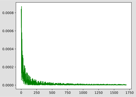
print(g.messageApproximationScheme())
print("--")

print("Temps de calcul : {0}".format(g.currentTime()))
print("Nombre d'itérations : {0}".format(g.nbrIterations()))

--
stopped with epsilon=1e-07
--
Temps de calcul : 4.026140166
Nombre d'itérations : 853000

In [11]:

p = plot(g.history(), "g")

../_images/notebooks_96-Tools_klForBns_21_0.svg

Animation of Gibbs KL

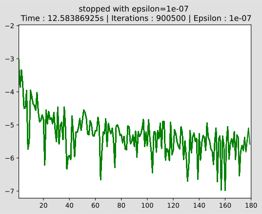
Since it may be difficult to know what happens during approximation algorithm, pyAgrum allows to follow the iteration using animated matplotlib figure

In [12]:

g = gum.GibbsBNdistance(bn, bn2)
g.setMaxTime(60)
g.setBurnIn(500)
g.setEpsilon(1e-7)
g.setPeriodSize(5000)

In [13]:

gnb.animApproximationScheme(g)  # logarithmique scale for Y
g.compute()

Out[13]:

{'klPQ': 2.4968819877105384,
 'errorPQ': 0,
 'klQP': 1.7185723934344816,
 'errorQP': 0,
 'hellinger': 0.7694372841144476,
 'bhattacharya': 0.3583810920680626,
 'jensen-shannon': 0.373998075835927}

../_images/notebooks_96-Tools_klForBns_25_1.svg